01 / 21

How quantum walks
see high-dimensional
structure

Quantum Walks on Simplicial Complexes and Harmonic Homology: Application to Topological Data Analysis with Superpolynomial Speedups

Authors

Ryu Hayakawa

Kyoto University

Kuo-Chin Chen

Foxconn Research

Min-Hsiu Hsieh

Foxconn Research

02 / 21

Problem

Graphs only capture pairwise interactions. The real shape of data is often higher-order.

Pairwise graph

Graphs represent observed pairwise links: which vertices are connected by selected edges.

Higher-dimensional object

Some correlations involve many points at once; representing them may require a higher-dimensional object.

03 / 21

Filtration

A filtration is a standard way to identify high-dimensional structure hidden in data.

From scale to structure

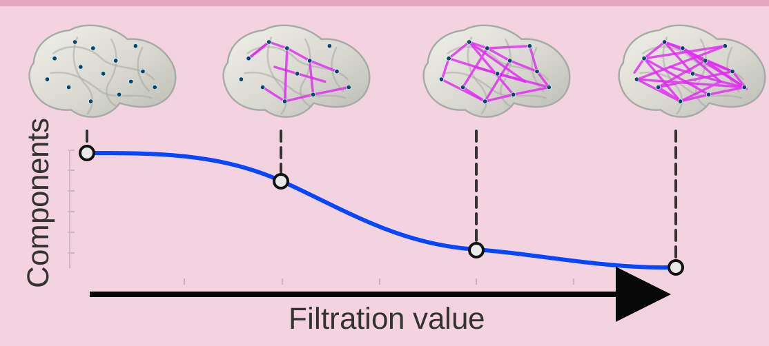
Instead of choosing one graph, grow a radius parameter. As scale increases, pairwise links, cycles, and filled higher-dimensional objects appear in a nested sequence.

Standard filtration picturescale increases left to right

04 / 21

Concrete example

Brain connectivity as a filtration example.

Brain connectivity study

Data

Brain regions become nodes; measured connectivity gives weighted links.

Filtration

Thresholds turn one weighted network into a nested sequence of complexes.

Signal

Cliques, loops, and higher-order holes become topological signatures, and these neuronal structures can be important for brain functionality.

Filtration value diagram with brain networks and decreasing components curve

05 / 21

Topological Data Analysis

TDA asks what survives as scale changes.

01

Start with a filtration

A filtration gives a nested sequence of complexes across radius or threshold.

02

Track birth and death

Components, cycles, voids, and higher-order holes appear, merge, fill, or disappear.

03

Return descriptors

Long-lived features become compact signatures of high-dimensional structure.

TDA goal

Separate stable high-dimensional signal from scale-specific noise.

06 / 21

Vocabulary bridge

Notation bridge: from X_k to β_k.

X_k

k-simplices

the set of all k-simplices

C_k, ∂_k

chains / boundary map

C_k = span(X_k)∂_k: C_k → C_k-1

Z_k, B_k

cycles / boundaries

Z_k = ker ∂_kB_k = im ∂_k+1

H_k

homology

the quotient group Z_k/B_k

β_k

Betti number

rank of H_k

07 / 21

Classical bottleneck

Why the main targets of TDA are hard classically.

β_k/|X_k|

Normalized Betti

RoleEstimate the normalized k-dimensional hole count on a comparable scale.

Classical bottleneckInverse-polynomial normalized Betti estimation is DQC1-hard for general simplicial complexes.

β^i,j_k/|X_k|

Persistent Betti

RoleEstimate the robust features that persist across filtration level i to level j.

Classical bottleneckNo known efficient inverse-polynomial estimator.

H_k(X(G))≠0?

Promise clique homology

RoleTurn a graph problem into asking whether the clique complex has nontrivial H_k.

Classical bottleneckThe promise clique homology problem is QMA₁-complete.

08 / 21

Main results

Quantum gate-count bounds.

β_k/|X_k|

Normalized Betti

Accuracyadditive error ±ε

Gate costO(n³ log(1/ε))×1/λ_k

Gapλ_k ∈ Ω(1/poly(n))

β^i,j_k/|X_k|

Persistent Betti

Accuracyadditive error ±ε

Gate costÕ(n³ log(1/ε))×(1/λ^i,down + 1/λ^j,up)

Gapλ^i,down, λ^j,up ∈ Ω(1/poly(n))

H_k(X(G))≠0?

Promise clique homology

DecisionYES ≥ 1 − O(ε); NO ≤ O(ε)

Gate costO(n³ log(1/ε))×1/g(n)

Gapg(n) ≥ 1/poly(n)

09 / 21

Technical contribution

Implementation costs behind the main gate bounds.

All three bounds use the same projector-building pattern.

U^up, U^down, U^h

Walk unitaries

RoleBuild the walk unitaries from graph adjacency.

Gate costÕ(n² log(1/ε))

ResultTheorem 4 gives an efficient implementation of the walk primitives.

Δ → Π

Laplacian + QSVT

RoleEncode the Laplacian and turn it into a projector.

Walk-unitary usesO(K log(1/ε))×1/λ_k

OutputK is the walk normalization factor; the projector depends on the application.

apply Π

Application readout

RoleAttach the target-specific readout to the projector.

Gate costO(n³ log(1/ε))×1/λ_k

BridgeThis is the reusable gate-count scale behind the application bounds.

10 / 21

Applications

High-dimensional Dirichlet: from boundary data to harmonic extension.

Given boundary values on a simplicial boundary, solve for a compatible interior signal with harmonic dynamics.

f_∂ ↦ u

Boundary-value problem

TaskSolve Δ_ku = 0 with fixed boundary data.

InputBoundary values f_∂ on boundary k-simplices.

GoalProduce an interior signal u that is harmonic with the prescribed boundary data.

Proj(ker Δ_k)

Article result

RoleBuild the harmonic projector with the walk unitary and QSVT.

Gate costO(n³ log(1/ε))×1/λ_k

GapNeed λ_k ∈ Ω(1/poly(n)).

11 / 21

Positioning

This is not merely another QTDA algorithm; it connects quantum walks to Hodge topology.

Classical picture

Recent classical work has built a genuine high-dimensional walk theory: up/down walks, Hodge Laplacians, and expander-style spectral analysis on simplicial complexes.
These tools already describe mixing, geometry, and topology beyond ordinary graph random walks.
So the real opening is not inventing high-dimensional structure from scratch, but carrying this mature picture into a quantum setting.

Earlier quantum picture

Earlier quantum TDA often focused on matrix-access models, generic linear-algebra speedups, or oracle-based routines.
Quantum walks on simplicial complexes existed, but their relation to harmonic homology was not yet the main message.
The link from graph adjacency all the way to TDA-ready homology readout was still missing.

This paper

Gives a rigorous relation between quantum walks and homology.
Encodes the combinatorial Laplacian through orientation interference.
Provides an efficient construction for clique complexes from graph adjacency.

12 / 21

Open directions

The most interesting next step is not just faster algorithms, but a richer language for how walks see topology.

Persistent Laplacian

Can we directly construct a quantum walk that projects onto persistent harmonic homology, rather than combining multiple projectors?

Beyond QSVT

Can quantum walk dynamics reveal low-energy or harmonic information without relying on QSVT?

High-dimensional expanders

Can the random-walk theory of high-dimensional expanders acquire a quantum counterpart?

Practical regimes

Which data families have efficient sampling, a reasonable gap, and a large enough normalized Betti signal?

13 / 21

Takeaway

Takeaway: one shared quantum pipeline turns hard TDA targets into explicit gate bounds.

Classical bottleneck

The three main TDA targets are already classically difficult: DQC1-hard, no known efficient inverse-polynomial estimator, and QMA₁-complete.

Main results

The paper gives explicit quantum gate-count bounds for all three targets, with additive accuracy and the expected inverse-gap penalties.

Technical bridge

All three bounds come from one reusable pipeline.

walk unitaries → Laplacian encodings → QSVT projectors → target readout

14 / 21

Technical details

The proof route is a five-step pipeline that the next slides unpack one by one.

STEP 1

Define walk states with orientation

Use signed simplex states so the Laplacian sign structure can be represented coherently.

σ ∈ X_kq ∈ {+,−}|σ,q⟩ ∈ span(X_k^±)

Paper mapSetup: §1.2, §3.2

STEP 2

Build U^up, U^down, U^h

Construct the up, down, and harmonic quantum walk unitaries from the oriented transitions.

U^up → P^upU^down → P^downU^h → P

Paper mapDefs. 2–4 (§3.2)

STEP 3

Turn walks into Laplacian encodings

Show these walk unitaries encode the relevant up, down, and full combinatorial Laplacians.

Δ_k^upΔ_k^downΔ_k

Paper mapProps. 1–3 (§3.2)

STEP 4

Use QSVT to build projectors

Apply QSVT to obtain projectors onto the topology-relevant subspaces.

Proj(Z^k)Proj(B_k)Proj(Z_k)Proj(B^k)Proj(ℋ_k)

Paper mapThm. 3 (§3.1)

STEP 5

Attach the application readout

Read out the quantity needed for normalized Betti, persistent Betti, or promise clique homology.

β_k/|X_k|β_k^i,j/|X_kⁱ|H_k(X(G)) = 0?

Paper mapThms. 5–7 (§5)

15 / 21

Technical move

Step 1: one geometric simplex becomes two orientation states.

state representation

|σ,q⟩ = |x_σ⟩ ⊗ |q⟩

Effect: the walk no longer sees only adjacency.It also carries whether a transition preserves or reverses orientation.

positive

q = + : positive orientation

negative

q = − : reversed orientation

SourceSetup §1.2, §3.2

16 / 21

Three walks

Step 2: build walks whose transition matrices encode the Laplacian pieces.

Up walk unitary encoding: U^up → P^up

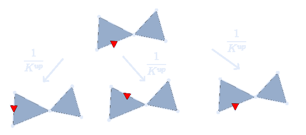
Move through a shared coface; this is the walk primitive for the up-Laplacian.

shared (k+1)-cofacetarget: Δ_k^up

SourceDefinition 2 (§3.2)

Down walk unitary encoding: U^down → P^down

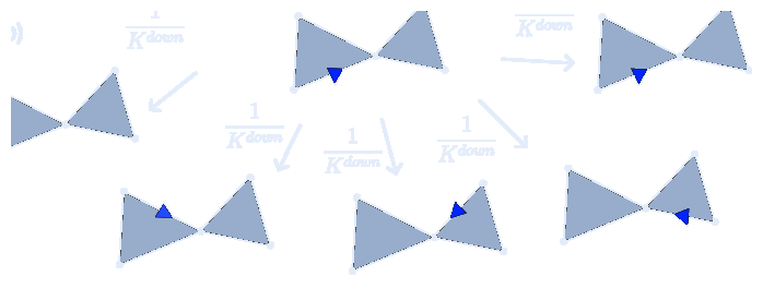
Move through a shared lower face; this is the walk primitive for the down-Laplacian.

shared (k−1)-facetarget: Δ_k^down

SourceDefinition 3 (§3.2)

Harmonic walk unitary encoding: U^h → P

Harmonic random walk panel from Figure 2

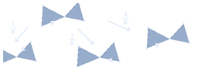
The harmonic walk encodes the full Δ_k used for kernel projection.

full Laplaciantarget: ℋ_k = ker Δ_k

SourceDefinition 4 (§3.2)

17 / 21

Algorithmic pipeline

Step 3: turn U^up, U^down, and U^h into Laplacian encodings.

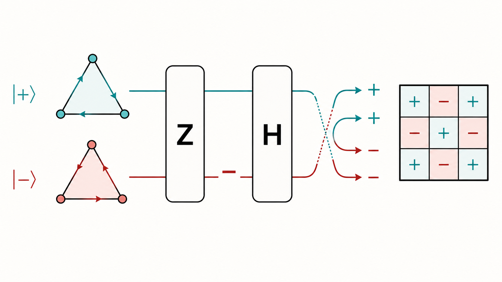
Orientation branches pass through Z then H to produce signed Laplacian-like matrix elements

INPUT

Projected walk encodings

Start from walk unitaries that encode Markov transition matrices.

U^up → P^up U^down → P^down U^h → P

SourceDefinitions 2–4

INTERFERENCE

Z marks; H interferes

In HZ, Z acts first on the orientation qubit; H mixes the signed branches.

Z: |−⟩ → −|−⟩ H: interfere ±

SourceProofs of Propositions 1–3

OUTPUT

Laplacian encodings

The signed transition rule becomes the encoded combinatorial Laplacian.

Δ_k^up Δ_k^down Δ_k

SourcePropositions 1–3

18 / 21

Efficient construction

Step 4: use QSVT on the encoded Laplacian to build the harmonic projector.

step input

Δ_k

Start with the encoded combinatorial Laplacian from Step 3.

Δ_k^up Δ_k^down

SourcePropositions 1–3

QSVT filter

p(Δ_k)

Use a polynomial filter for the zero eigenspace.

p(0) ≈ 1 p(x ≥ λ_k) ≈ 0

SourceTheorem 3

implementation cost

O(log(1/ε)) / λ_k

Calls to the encoded walk unitary.

SourceTheorem 3

step 4 result

Proj(ℋ_k)

A shared harmonic projector primitive, before any application-specific readout.

ℋ_k = ker Δ_k zero modes

SourceTheorem 3

shared primitive gate count

O(n³ log(1/ε)) / λ_k

walk construction cost times QSVT calls

SourceTheorem 3

19 / 21

Target readout

Step 5: attach the application-specific readout.

Normalized Bettiβ_k / |X_k|Projector readoutestimate Tr(Proj(ℋ_k)) / |X_k|Extra ingredientuniform k-simplex sampling

SourceTheorem 5

Persistent Bettiβ_k^i,j / |X_kⁱ|Projector readoutcombine Proj(Z_kⁱ) with Proj(B_k^j)Filtration rolecycles born by i, boundaries by j

SourceTheorem 6

Promise clique homologyH_k(X(G)) = 0 ?Projector readouttest whether Proj(ker Δ_k) has supportOutputYES/NO under the promise gap

SourceTheorem 7

Same machinery QSVT builds the needed projectors; each target chooses a different readout.

20 / 21

Assumption map

What assumptions attach to the three results?

Normalized Bettiλ_k + X_k accessgap for projectoruniform simplex sampling for readout

Persistent Bettiλ^i,down, λ^j,up + X_kⁱ accesstwo gap termsuniform sampling at filtration level i

Promise clique homologyNO-case gap g(n)λ_min(Δ_k) ≥ g(n)

Key point gap terms drive projector cost; simplex sampling enters only the Betti readout.

21 / 21

KYOTO UNIVERSITY X FOXCONN RESEARCH

Thank you!

Source: Quantum 10, 2138 (2026).

QUESTIONS?

How quantum walkssee high-dimensionalstructure

Graphs only capture pairwise interactions. The real shape of data is often higher-order.

A filtration is a standard way to identify high-dimensional structure hidden in data.

Brain connectivity as a filtration example.

TDA asks what survives as scale changes.

Start with a filtration

Track birth and death

Return descriptors

Notation bridge: from Xk to βk.

Why the main targets of TDA are hard classically.

Quantum gate-count bounds.

Implementation costs behind the main gate bounds.

High-dimensional Dirichlet: from boundary data to harmonic extension.

This is not merely another QTDA algorithm; it connects quantum walks to Hodge topology.

Classical picture

Earlier quantum picture

This paper

The most interesting next step is not just faster algorithms, but a richer language for how walks see topology.

Persistent Laplacian

Beyond QSVT

High-dimensional expanders

Practical regimes

Takeaway: one shared quantum pipeline turns hard TDA targets into explicit gate bounds.

The proof route is a five-step pipeline that the next slides unpack one by one.

Define walk states with orientation

Build Uup, Udown, Uh

Turn walks into Laplacian encodings

Use QSVT to build projectors

Attach the application readout

Step 1: one geometric simplex becomes two orientation states.

Step 2: build walks whose transition matrices encode the Laplacian pieces.

Step 3: turn Uup, Udown, and Uh into Laplacian encodings.

Projected walk encodings

Z marks; H interferes

Laplacian encodings

Step 4: use QSVT on the encoded Laplacian to build the harmonic projector.

Step 5: attach the application-specific readout.

What assumptions attach to the three results?

Thank you!

How quantum walks
see high-dimensional
structure

Notation bridge: from X_k to β_k.

Build U^up, U^down, U^h

Step 3: turn U^up, U^down, and U^h into Laplacian encodings.